
From EKF-SLAM to iSAM2 - Part 2 (FastSLAM)
1 · SLAM at Scale
In the previous post, we ended with the scaling limits of EKF‑SLAM: both memory and per‑update computation grow quadratically with the number of poses and landmarks. For demanding applications that need accurate, large‑area maps like those required by autonomous 3‑D inspections1, the environment may contain tens of thousands to millions of landmarks. The SLAM backbone for navigation and planning must scale accordingly.
In this post, we focus on FastSLAM, a particle‑filtering framework that exploits SLAM’s conditional‑independence structure. For several years, FastSLAM was the most popular academic SLAM approach.
FastSLAM also paved the way for GMapping 2, one of ROS’s most widely used open‑source SLAM packages. Although often viewed as “old‑school,” it remains a practical, plug‑and‑play option nearly two decades after its release.
1.1 · FastSLAM Highlights
- Computational efficiency. A straightforward implementation costs $\mathcal O(NL)$ for $N$ particles and $L$ landmarks using a Rao‑Blackwellized Particle Filter (RBPF); tree‑based data structures reduce average access to $\mathcal O(\log L)$, yielding about $\mathcal O(N\log L)$ per update.
- Robust data association. Multiple hypotheses are maintained across particles, mitigating the catastrophic failures common in EKF‑SLAM when associations are wrong.
2 · Monte Carlo Estimation and Particle-Based Representations
Monte Carlo methods are widely used across science and engineering. Monte Carlo 3 refers to estimating quantities of interest (often integrals) by random sampling:
Monte Carlo integration. For a domain $V\subseteq\mathbb R^s$, an integrand $f$, and a sampling density $p$,
\[\int_V f(x)\,dx = \int_V p(x)\,\frac{f(x)}{p(x)}\,dx \approx \frac1N\sum_{i=1}^N \frac{f(x_i)}{p(x_i)},\quad x_i\sim p.\]
2.1 · Particle (Empirical) Approximations
We denote by $x_k$ the robot state at time $k$, by $u_{k-1}$ the control applied between $k{-}1$ and $k$, and by $z_k$ the measurement at time $k$. Let $x_{0:k}=(x_0,\dots,x_k)$ be the trajectory up to time $k$. Our goal is to approximate the posterior $p(x_{0:k}\mid z_{1:k},u_{1:k-1})$.
A particle approximation represents a distribution by $N$ weighted samples $(w_k^{(i)},x_{0:k}^{(i)}) _ {i=1}^N$ with $\sum_{i=1}^N w_k^{(i)}=1$. Using the Dirac delta $\delta(\cdot)$, the empirical measure is
\[\widehat{p} _ k (x _ {0:k} \mid z _ {1:k}, u _ {1:k-1}) = \sum _ {i=1} ^{N} w _ k^{(i)} \, \delta(x _ {0:k} - x _ {0:k} ^{(i)}).\]For any integrable function $g$, expectations become weighted sample averages:
\[\mathbb{E} _ {x _ {0:k} \sim \widehat{p}} [g(x _ {0:k})] = \sum _ {i=1} ^{N} w _ k^{(i)} \, g(x _ {0:k} ^{(i)}).\]2.2 · Sequential Particle Filtering (SIS/SIR)
Sequential filtering incrementally updates the particle approximation of our posterior. At each time step we use only the previous estimate and new data, rather than revisiting the full history. Still, this update accounts for all past controls and measurements. Particle filtering has a deep mathematical foundation; for details see Doucet et al. 4.
We assume probabilistic models for how the robot moves and senses:
- Prior $p(x _ 0)$: initial state distribution.
- Motion model $p(x _ k \mid x _ {k-1}, u _ {k-1})$: how the state evolves under control.
- Sensor model $p(z _ k \mid x _ k)$: likelihood of the measurement given the state.
- Proposal $q _ k(x _ k \mid x _ {k-1}, u _ {k-1}, z _ k)$: the distribution from which we actually sample new states. A common and simple choice is $q _ k = p(x _ k \mid x _ {k-1}, u _ {k-1})$.
Why do we need a proposal?
If we could sample directly from the posterior over trajectories and maps, particle filtering would be trivial. But this is exactly the intractable distribution we aim to approximate!
Instead, we sample from a more convenient distribution $q _ k$ and correct with importance weights.
SIS (Sequential Importance Sampling)
At each time $k$ and for each particle $i$:
- Propagate (sample): draw $x _ k^{(i)} \sim q_k(\cdot \mid x _ {k-1}^{(i)}, u _ {k-1}, z _ k)$.
-
Reweight:
\[\tilde w _ k^{(i)} = w _ {k-1}^{(i)} \cdot \frac{\underbrace{p(z _ k \mid x _ k^{(i)})} _ {\text{sensor likelihood}} \,\underbrace{p(x _ k^{(i)} \mid x _ {k-1}^{(i)}, u _ {k-1})} _ {\text{motion prior}}} {\underbrace{q _ k(x _ k^{(i)} \mid x _ {k-1}^{(i)}, u _ {k-1}, z _ k)} _ {\text{proposal}}}, \quad w _ k^{(i)} = \frac{\tilde w _ k^{(i)}}{\sum _ j \tilde w _ k^{(j)}}.\]For $q _ k = p(x _ k \mid x _ {k-1}, u _ {k-1})$, the (unnormalized) importance weight simplifies to the observation likelihood:
\[\tilde w _ k^{(i)} = p(z _ k \mid x _ k^{(i)}).\]
SIR (Sequential Importance Resampling)
Over time, particle weights concentrate on a few particles, a phenomenon called degeneracy. SIR addresses this by resampling:
\[x _ k ^{(i)} \sim \text{Cat}\{w _ k^{(i)}\}_{i=1}^N,\]and resetting $w _ k^{(i)} = 1/N$. This reallocates computational effort to high-probability regions.
The combination of motion-model proposals with resampling is known as the bootstrap filter.
When to resample?
- A simple rule is to resample at every step.
-
A more effective approach is to resample when the effective sample size (ESS)
\[\widehat{N} _ {\mathrm{eff}} = \frac{1}{\sum_i (w _ k^{(i)})^2}\]falls below a threshold $N_T$. Typically $0.3N \leq N_T \leq 0.7N$.
Why Plain SIR Struggles for SLAM
The required number of particles grows exponentially with state dimension 5. Even for localization, a ground robot may need to represent a 3-DOF (2-D) or 6-DOF (3-D) state. Adding thousands of landmark variables to estimate the full SLAM posterior $p(x _ {0:k}, m^{1:L} \mid z _ {1:k}, u _ {1:k-1})$ makes plain SIR impractical. The key idea of Rao-Blackwellization (next section) is to sample only the trajectory and integrate out the map.
3 · Factored Representation of SLAM
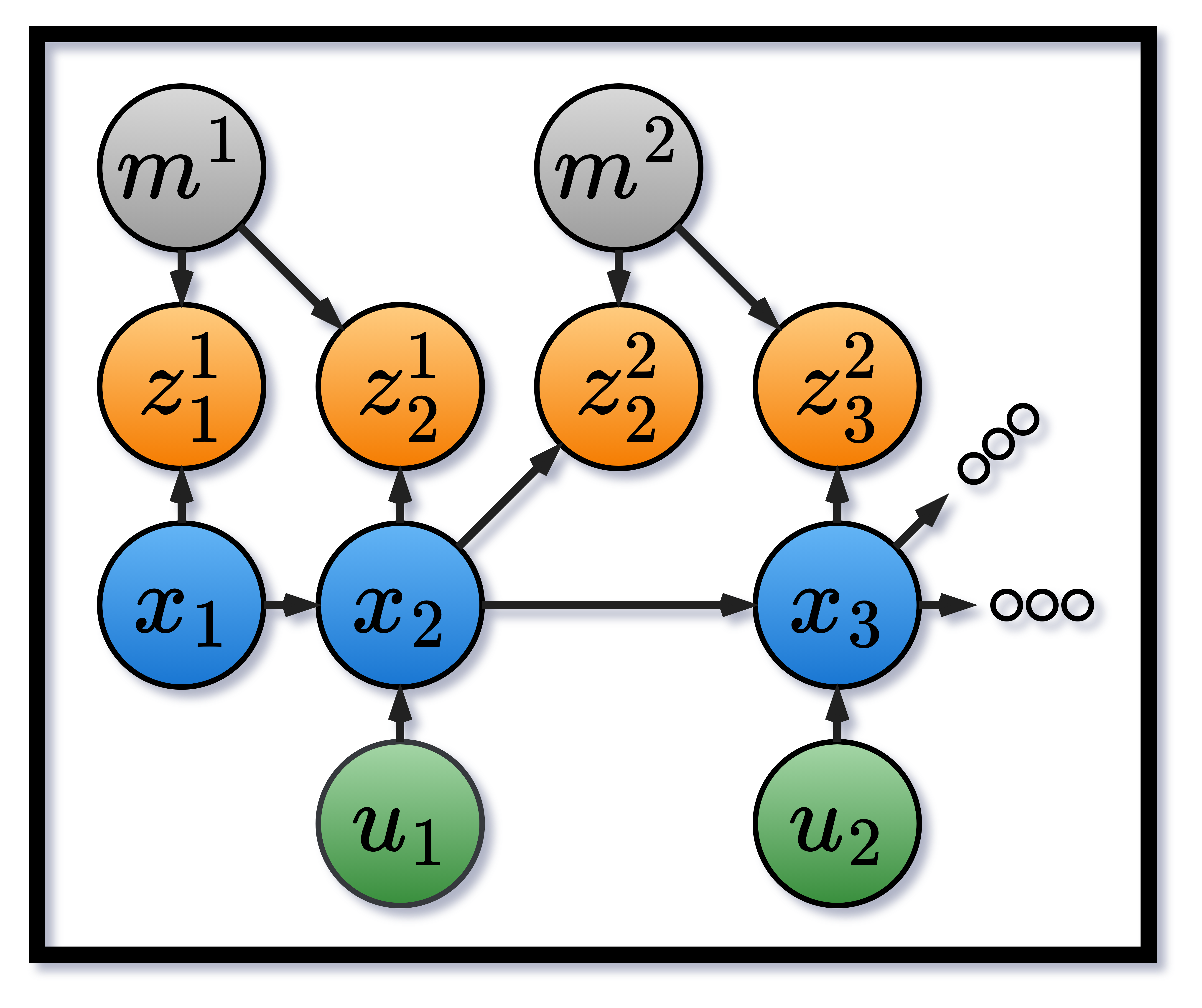
Notation. Let $z _ {1:k}$ be measurements, $u _ {1:k-1}$ controls, $x _ {0:k}$ the trajectory, and $m^{1:L}$ the (static) landmark map.
One of the major insights that led to the development of efficient SLAM algorithms is that the posterior factorizes as:
\[p(x_{0:k}, m^{1:L} \mid z_{1:k}, u_{1:k-1}) = p(m^{1:L} \mid x_{0:k}, z_{1:k}) \cdot p(x_{0:k} \mid z_{1:k}, u_{1:k-1}).\]And specifically FastSLAM introduced the insight that given the entire path $x_{0:k}$, the map posterior $p(m^{1:L} \mid x_{0:k}, z_{1:k})$ decouples across landmarks (with known data association):
\[p(m^{1:L} \mid x_{0:k}, z_{1:k}) = \prod_{i=1}^L p(m^i \mid x_{0:k}, z^i_{1:k}),\]where $z^i_{1:k}$ denotes the subsequence of measurements of landmark $i$. The fully factored posterior is therefore:
\[p(x_{0:k} \mid z_{1:k}, u_{1:k-1}) \cdot \prod_{i=1}^L p(m^i \mid x_{0:k}, z^i_{1:k}).\]This “simple” result can be easily missed, but it implies a lot - if we know the entire pose history, the posterior of each landmark becomes simple to estimate, as each landmark can be estimated independently as a product of simple measurement models.
Let’s assume for now that we know the pose variables $x_{0:k}$. We’ll get back to this later.
3.1 · Landmark Posteriors
For a single landmark $m^i$, the recursive update is
\[p(m^i \mid x_{0:k}, z^i_{1:k}) = \eta \, p(z^i_k \mid x_k, m^i) \, p(m^i \mid x_{0:k-1}, z^i_{1:k-1}),\]where $\eta$ is a normalizer independent of $m^i$.
Following our previous post, we can use the EKF to maintain Gaussian landmark posteriors:
- Assume $p(m^i \mid x_{0:k-1}, z^i_{1:k-1}) = \mathcal{N}(\mu_{k-1}^i, \Sigma_{k-1}^i)$.
- Assume the measurement model $z^i_k = h(x_k, m^i) + w_k^i$, with $w_k^i \sim \mathcal{N}(0, R_k^i)$.
Each landmark update is then an EKF step, independent across landmarks, and we obtain constant complexity per landmark.
In practice, we do not know the trajectory $x_{0:k}$. To exploit this factorization, we use Particle Filters and specifically the Rao-Blackwellized Particle Filter (RBPF). By sampling trajectories and weighting them by measurement likelihoods, the particle set tracks the true trajectory distribution with high probability 6.
3.2 · Rao-Blackwellization for SLAM
RBPF in one line: sample the hard part (the trajectory), integrate the easy part (landmarks) analytically.
In RBPF we represent $p(x_{0:k} \mid z_{1:k}, u_{1:k-1})$ with particles. For each particle, we maintain independent EKF landmark filters conditioned on that trajectory.
In the bootstrap filter, the importance weight update simplifies to $\tilde w_k^{(i)} = p(z_k \mid x_k^{(i)})$. For SLAM, we refine this using the landmark factorization:
\[p(z_k^i \mid x_{0:k}^{(i)}, z_{1:k-1}^i) = \eta \int p(z_k^i \mid m^i, x_k^{(i)}) \, p(m^i \mid x_{0:k-1}^{(i)}, z_{1:k-1}^i) \, dm^i.\]Both terms are Gaussian, so this integral is analytic. The result uses standard EKF quantities:
\[\tilde w _ k^{(i)} = |2 \pi Q_k^{(i)}|^{-1/2} \exp\left(-\tfrac12 (z_k^i - \hat z_k^i)^T (Q_k^{(i)})^{-1} (z_k^i - \hat z_k^i)\right),\]with
\[\hat z_k^i = h(x_k^{(i)}, \mu^{i,(i)}), \qquad Q_k^{(i)} = \left(\frac{\partial h}{\partial x}\Big|_{x_k^{(i)}, \mu^{i,(i)}}\right)^T \Sigma_k^{i,(i)} \left(\frac{\partial h}{\partial x}\Big|_{x_k^{(i)}, \mu^{i,(i)}}\right).\]These terms are already computed during the EKF update, so evaluating the weight is efficient.
3.3 · Why Rao-Blackwellization Helps
Instead of sampling landmarks, we integrate them out analytically:
- Variance reduction. By the law of total variance, Rao-Blackwellization strictly lowers estimator variance compared to joint sampling of $(x, m)$.
- Lower complexity. Sampling in $(x_{0:k}, m^{1:L})$ would require exponentially more particles. Integrating landmarks keeps the filter tractable.
- Gaussian structure. Each landmark is stored compactly as $(\mu, \Sigma)$ and updated independently, avoiding the curse of dimensionality.
4 · FastSLAM 1.0 - Step by Step
FastSLAM in its original form (later called FastSLAM 1.0) was introduced in 2002 7. Many subsequent improvements built on this foundation.
4.1 · Simplified Algorithm
We now assemble the pieces into a simplified version of FastSLAM 1.07:
- Initialization. Create particles, each with a trajectory and per-landmark Gaussian estimates: $\big(x_{0:k}^{(i)}, \mu_k^{1,(i)}, \Sigma_k^{1,(i)}, \dots, \mu_k^{L,(i)}, \Sigma_k^{L,(i)}\big)$.
- Prediction. For control $u_{k+1}$, propagate each trajectory to obtain $x_{0:k+1}^{(i)}$.
-
Update. For each particle:
- Perform an EKF update of each observed landmark.
- Compute the particle weight $w_k^{(i)}$ as the product of observation likelihoods (often accumulated in log form for stability).
- Resampling. Draw a new set of particles with probability proportional to $w_k^{(i)}$.
4.2 · Toward the Full Algorithm
To make FastSLAM practical and robust for online use, several additional mechanisms are required. The full details are presented in the extended paper 8. Here we highlight the most important elements.
Data Association
So far, we assumed known correspondences $z_k^i$ (which landmark produced which measurement). In practice, correspondences must be inferred. FastSLAM handles this by assigning each observation to the most likely landmark, i.e. the one maximizing the measurement likelihood under its current Gaussian estimate and sensor model. This procedure mirrors the calculation used for importance weights.
Conceptually, the algorithm “guesses” correspondences, and resampling ensures that particles with good guesses persist while others die out.
Efficient Landmark Management
Naively copying landmark estimates for each particle at every step would be too expensive. Instead, FastSLAM uses tree-based data structures to avoid unnecessary duplication. Access to a landmark among $L$ requires only $\log L$ operations, and since only a small subset of landmarks is observed at each step, the update cost per iteration is $\mathcal O(N \log L)$.
Per-Particle Data Association
Each particle maintains its own correspondence hypotheses. This diversity allows the filter to handle ambiguous or incorrect associations more gracefully than EKF-SLAM, where a single wrong association can cause catastrophic failures.
5 · FastSLAM 2.0 and GMapping
FastSLAM 2.0 8 improved on FastSLAM 1.0 by introducing a better proposal distribution. Instead of sampling the next pose from the motion model alone, it incorporates the latest scan $z_k$ (via scan matching) to approximate $p(x_k \mid x_{k-1}, u_{k-1}, z_k)$. This reduces weight variance and lowers the number of required particles.
FastSLAM 2.0 is definitely more involved than its predecessor - if you manage to understand it, then you’re a true probabilistic robotics master!
5.1 · Occupancy Grids vs. Landmark Maps
While landmark-based maps estimate continuous positions $m^i$, occupancy grids discretize the world into independent Bernoulli cells $m^j \in {0,1}$. Given a trajectory $x_{0:k}$, cells update independently using log-odds from the range sensor model. This formulation is efficient: particles represent trajectories only, while maps are updated deterministically per particle.
The grid representation trades geometric accuracy for robustness and speed. Landmarks provide compact, continuous estimates but require explicit data association. Grids avoid this by treating the environment as a dense array of cells, at the cost of higher memory usage.
5.2 · GridSLAM and Its Advantages
This occupancy-grid formulation, combined with RBPF, is often called GridSLAM. It became the dominant approach for 2-D LiDAR mapping because it offers:
- Simple sensor models with fast per-cell updates.
- Scan matching to produce accurate proposals for $x_k$.
- Per-particle data association that tolerates ambiguity.
5.3 · GMapping
GMapping 2 built directly on GridSLAM, adding several practical enhancements:
- Improved proposals (FastSLAM 2.0 style): use scan matching with $z_k$ for better sampling.
- Grid-based mapping: occupancy grids updated in log-odds, implemented efficiently.
- Selective resampling: triggered only when effective sample size falls too low, reducing particle impoverishment.
- Robust scan matching: multi-resolution methods stabilize proposals and yield sharper maps in real time.
GMapping became one of the most widely used ROS SLAM packages. Even today, it remains a common baseline for 2-D mapping tasks.
Relevant links:
6 · Looking Towards GraphSLAM
FastSLAM and particle-based mapping were the first approaches to demonstrate practical, real-time SLAM at scale. At the time, many researchers considered the problem essentially solved:
“In general Rao-Blackwellized filters make for the most efficient SLAM algorithms.” 9
“While there are still many practical issues to overcome, especially in more complex outdoor environments, the general SLAM method is now a well understood and established part of robotics.” 10
In hindsight, these predictions did not age well. Just as Prof. von Jolly’s famous claim about the “end of theoretical physics” turned out to be premature, SLAM research was far from finished. During the same period, graph-based approaches matured rapidly and soon became the foundation of the most efficient and practical 3-D SLAM systems available today.
Stay tuned for the next chapter!
-
Links are for illustration only; there’s no sponsorship involved. ↩
-
Giorgio Grisetti, Cyrill Stachniss, and Wolfram Burgard. Improving Grid-based SLAM with Rao-Blackwellized Particle Filters by Adaptive Proposals and Selective Resampling. In Proc. IEEE ICRA, 2005. ↩ ↩2
-
Christiane Lemieux. Monte Carlo and Quasi-Monte Carlo Sampling. Springer, 2009. doi. ↩
-
A. Doucet, N. J. Gordon, and V. Krishnamurthy. Particle Filters for State Estimation of Jump Markov Linear Systems. Signal Processing 49(3), 2001: 613-624. ↩
-
Murphy, Kevin P. “Bayesian map learning in dynamic environments.” Advances in neural information processing systems 12 (1999). ↩
-
Murphy, Kevin, and Stuart Russell. Rao-Blackwellised Particle Filtering for Dynamic Bayesian Networks. In Sequential Monte Carlo Methods in Practice, Springer, 2001. ↩
-
Montemerlo, Michael, Sebastian Thrun, Daphne Koller, and Ben Wegbreit. “FastSLAM: A factored solution to the simultaneous localization and mapping problem.” AAAI (2002): 593‑598. ↩ ↩2
-
Thrun, Sebastian, Michael Montemerlo, Daphne Koller, Ben Wegbreit, Juan Nieto, and Eduardo Nebot. “Fastslam: An efficient solution to the simultaneous localization and mapping problem with unknown data association.” Journal of Machine Learning Research 4, no. 3 (2004): 380-407. ↩ ↩2
-
Drew Bagnell and Bryan Wagenknecht: SLAM, Fast SLAM, and Rao-Blackwellization. In Statistical Techniques in Robotics (16-831, F09), Lecture #24 (November 12, 2009). link ↩
-
Durrant-Whyte, Hugh, and Tim Bailey. “Simultaneous localization and mapping: part I.” IEEE Robotics & Automation Magazine 13(2), 2006: 99‑110. ↩