
From EKF-SLAM to iSAM2 - Part 1
1 · Why we need good mapping algorithms
Ever wondered how your robot vacuum knows where it’s been, and where it still needs to go?
Before any smart system can decide what to do next, it must picture the world around it. That picture begins with mapping: stitching noisy sensor flashes into a single, always-evolving map of the surroundings.
Why is mapping so valuable?
- Plan smarter: a clear map lets the robot choose obstacle-free, shorter paths instead of wandering blind.
- Remember better: as the map refines, tomorrow’s route improves automatically.
- Share data: a well-built map can live on; teammates (or humans) can reuse it for their own tasks.
And mapping isn’t just for vacuums. Real-time 3-D maps now power: 1
- Self-flying camera drones keeping athletes in frame.
- Autonomous forklifts weaving through warehouses.
- Automated crop harvesting in orchards.
- Even niche uses like robot parkour.
In short: if a machine moves and senses, mapping is the secret sauce that makes the rest of the recipe possible.
This series From EKF-SLAM to iSAM2 explores the ingredients that make this possible, starting with the forerunner of modern approaches: EKF-SLAM.
2 · What is SLAM?
© Steve Macenski, LGPL 2.1. Original at GitHub.
SLAM or Simultaneous Localization and Mapping is a class of algorithms that let a robot:
- Localize - work out where it is in space.
- Map - work out what is around it.
The catch? Both tasks depend on each other: If you already know the map, you can triangulate your pose from landmarks; conversely, if you already know the pose, you can infer landmark positions. Drop a robot into an unfamiliar building and it has neither - hence the classic chicken-and-egg of robotics.
A quick refresher
- Localization - estimating the robot’s pose inside a known map.
Example: a GPS-guided car fuses satellite fixes with a road map to decide which lane it occupies. - Mapping - estimating landmark positions from a known pose.
Example: satellites in known orbits stitch overlapping images into the seamless world maps you browse online.
SLAM tackles the joint problem: update both pose and map online as new sensor data streams in.
Core intuition
The best pose is the one that makes the map consistent,
and the best map is the one that makes the poses consistent.
Viewed through today’s “data-centric” lens, this feels natural: more data leads to better estimates.
But in the 1980s the idea of coupling the two problems tightly was radical; researchers were used to solving them in separate phases.
In the next section we’ll see how the Extended Kalman Filter (EKF) became the first widely adopted framework to put that intuition into practice, and how it launched SLAM research into high gear.
3 · EKF-SLAM
The term SLAM took off after Dissanayake et al. 2 published a 2001 paper that gathered two decades of scattered ideas into one recipe: Extended Kalman-Filter SLAM, or EKF-SLAM. They showed how a single estimator can track both the robot pose and every landmark at once. EKF-SLAM tracks a huge cloud of uncertainty that covers the robot pose and every landmark, as gradually “tightening” with each observation.
They proved several useful mathematical properties of how this uncertainty behaves in the paper.
- Theorem 1: Landmark uncertainty never increases with more observations.
- Theorem 2: As the number of observations grows, estimates of different landmarks become perfectly correlated. At perfect correlation, knowing the exact position of one immediately implies the other’s.
- Theorem 3: The smallest possible covariance for any single landmark is limited solely by the robot-pose uncertainty it had when that landmark first entered the map. Consequence: if we want to pin-point a landmark in global coordinates, we first need to know where the robot is in the global frame.
Why bring the EKF into SLAM?
SLAM is never exact. Sensors are noisy, readings can clash, and sometimes nothing is observed at all. The Extended Kalman Filter (EKF) is a classic way to fuse such imperfect information. The algorithm consists of two steps:
- Predict the state forward in time with the “motion model” - a function describing the change in time.
- Update that prediction using fresh measurements, weighted by their reliability (i.e. uncertainty).
EKF-SLAM runs those two steps on a joint state, that contains both the robot pose and the full landmark map. Treating them together is critical: an improved landmark estimate immediately tightens the pose uncertainty, and a better pose does the same for every landmark. Dropping these cross-correlations would throw away valuable information.
In the algorithm, predict handles robot motion, while update folds in the latest sensor readings. The landmarks themselves are assumed stationary, so only the pose block receives motion noise.
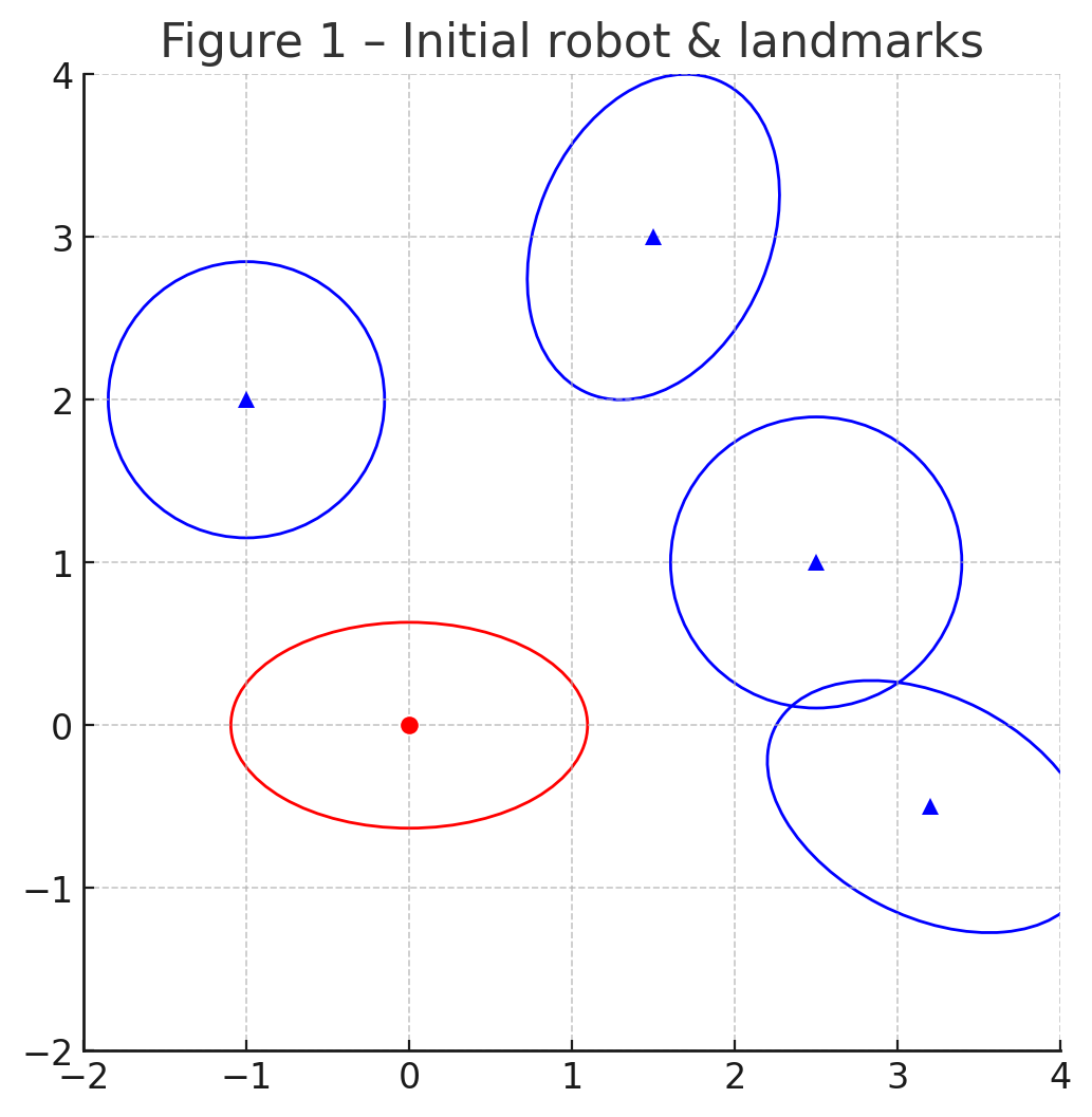
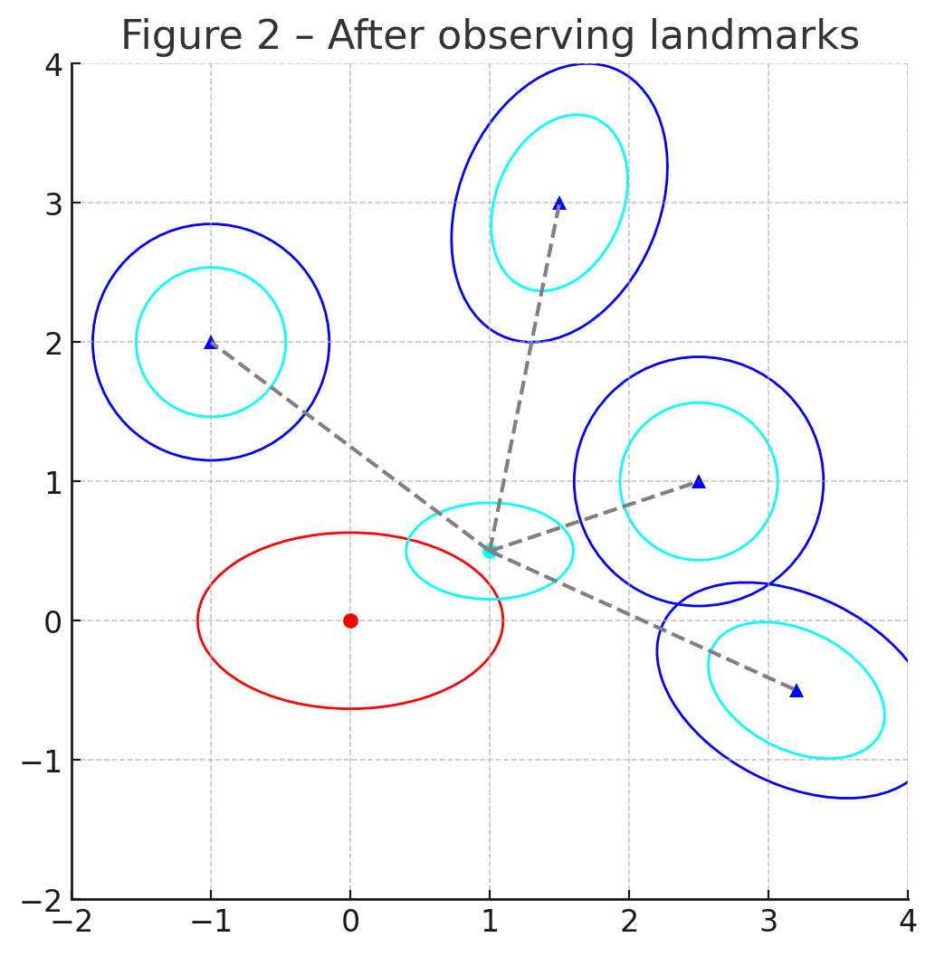
Left: initial uncertainty for the robot (red ellipse) and four landmarks (blue).
Right: after one scan the ellipses shrink (cyan) because the update step couples pose and landmarks through the same Kalman gain.
Mathematical formulation
The Kalman Filter maintains the posterior $p(\mathbf{x} _ {k} \mid \mathbf{z} _ {1:k})$ - the best Gaussian estimate of the current state after all measurements up to time $k$.
With linear models that posterior is exact; the Extended KF linearizes the motion/measurement models around the current estimate, so the same algorithm still works when they are mildly non-linear.
We stack the robot pose and all $N$ landmarks into $\mathbf{y} _ k = [\,\mathbf{x}_k^\top\;\mathbf{m} _ k^\top\,]^\top$ and track its covariance $\mathbf{P} _ k$.
State transition
The robot moves according to
\[\mathbf{x} _ {k+1}=f(\mathbf{x} _ k,\mathbf{u} _ k) + \mathbf{v} _ k, \qquad \mathbf{v} _ k\sim\mathcal{N}(\mathbf{0},\mathbf{Q} _ k),\]while landmarks stay put:
\[\mathbf{m} _ {k+1}=\mathbf{m} _ k.\]Written together,
\[\begin{bmatrix} \mathbf{x} _ {k+1}\\\mathbf{m} _ {k+1} \end{bmatrix}= \begin{bmatrix} f(\mathbf{x} _ k,\mathbf{u} _ k)\\\mathbf{m} _ k \end{bmatrix}+ \begin{bmatrix} \mathbf{v} _ k\\\mathbf{0} \end{bmatrix}.\]Predict step
Notes:
- The Jacobian is block-sparse:
- Noise $\mathbf{Q}_k$ affects only the pose block; landmarks inherit no motion noise.
Update step for one landmark $j$
A measurement delivers range/bearing (or a pixel, etc.)
\[\mathbf{z} _ {k,j}=h_j(\mathbf{x} _ k,\mathbf{p} _ j)+\mathbf{w} _ {k,j}, \qquad \mathbf{w} _ {k,j}\sim\mathcal{N}(\mathbf{0},\mathbf{R} _ {k,j}).\]Example: 2-D LiDAR
For a pose $\mathbf{x} _ k=[x_k,\,y_k,\,\theta_k]^\top$ and landmark $\mathbf{p} _ j=[p_{jx},\,p_{jy}]^\top$:
\[h_j(\mathbf{x} _ k)= \begin{bmatrix} \sqrt{(p_{jx}-x_k)^2+(p_{jy}-y_k)^2}\\ \operatorname{atan2}(p_{jy}-y_k,\,p_{jx}-x_k)-\theta_k \end{bmatrix}.\]We linearize $h_j$ to get $\mathbf{H}_{k,j}$ and apply the EKF formulas:
Notes:
- $\mathbf{H}_{k,j}=\partial h_j/\partial\mathbf{y}$ evaluated at the predicted state.
- The Kalman gain $\mathbf{K}_{k,j}$ couples pose and every landmark, so one new range/bearing tightens all map correlations.
- This is often implemented by looping over all measurements j. This keeps $\mathbf{S} _ {k,j}$ low dimensional, keeping the inversion cost small while exploiting the sparse structure of SLAM.
Putting it together
- Predict1 - propagate pose, drag the map along.
- For each new observation: Update2 - refine the joint state.
Everything else from data association, landmark initialization, to sparsity tricks, wraps around these two lines.
4 · Yet we rarely see EKF-SLAM anymore
EKF-SLAM solved the chicken-and-egg, but created an elephant-in-the-room matrix. As the map grows the covariance matrix fills in, so each predict and update step costs quadratic time $O(N^2)$, and the filter must store the same quadratic amount of memory - painful if you hope to map tens of thousands of landmarks.
A second computational challenge is in knowing “which dot is which” - assigning each measurement to the correct landmark, also known as data association. Wrong data association often causes catastrophic SLAM failures - ever seen your robot steer straight into a wall? I did…
Later methods attack these two limitations from different angles:
- FastSLAM breaks the map into particle-wise mini EKFs, so each landmark stays independent given one robot trajectory.
- iSAM2 turns SLAM into a sparse linear-algebra problem without sacrificing memory of the entire pose history, while keeping updates sparse and efficient.
Those improvements are the focus of the next posts in this series.